Profiling
Can I speed up my program?
Introduction
Are you in the situation where you wrote a program or script which worked well on a test case but now that you scale up your ambition, your jobs are taking an age to run? If so, then the information below is for you!
A Winning Strategy

The tried-and-tested formula involves asking the following questions:
Am I using the best algorithm for my task?
The reason why consideration of algorithms and data structures are top of the list is because changes to these typically offer the most benefit. An example of choosing a better algorithm is the comparison of an LU decomposition vs. an iterative method to solve a system of linear equations that result in a sparse matrix:

Can I improve the design of my data structures?
For a data structure example, compare the access time for a has table, which is O(1), to that of looking through each item in an array or list, O(N) for N items inspected. Thus if your code performs many lookups, you may want to investigate the use of alternative data structures.
Looking through all the cells of an array: O(N).
Binary search: O(logN).
Accessing an item in a hash table: O(1).


Which parts of my program take up most of the execution time?
Only after you have determined that you are using the best possible algorithm should you start to consider the way in which your algorithm is implemented. If you proceed to considering implementation, you will want to make sure you focus your efforts, and to do that, you will need to carefully analyse where your program is spending time. Just guessing at where your program is spending time is often a recipe for disappointment and frustration.

Now that I've found the hotspots, what can I do about them?
We'll get onto answering this question anon. First, however, it is essential that we go into battle fully informed. The next section outlines some key concepts when thinking about program performance. These will help focus our minds when we go looking for opportunities for a speed-up.
Factors which Impact on Performance
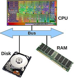
The Memory Hierarchy
These days, it takes much more time to move some data from main memory to the processor, than it does to perform operations on that data. In order to combat this imbalance, computer designers have created intermediate caches for data between the processor and main memory. Data stored at these staging posts may be accessed much more quickly than that in main memory. However, there is a trade-off, and caches have much less storage capacity than main memory.
The hip bone's connected to the...
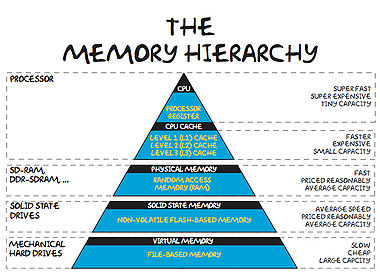
The memory hierarchy. From the small and fast to the large and slow.
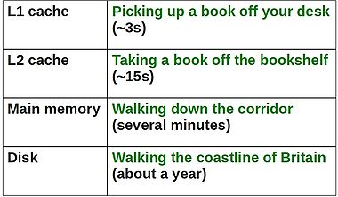
Translating nanoseconds to something we can visualise.


Now, it is clear that a program which is able to find the data it needs in cache will run much faster than one which regularly reads data from main memory (or worse still, disk).
Optimising Compilers
Compilers take the (often English-like) source code that we write and convert it into a binary code that can be comprehended by a computer. However, this is no trivial translation. Modern optimising compilers can essentially re-write large chunks of your code, keeping it semantically the same, but in a form which will execute much, much faster (we'll see examples below). To give some examples, they will split or join loops; they will hoist repeated, invariant calculations out of loops; re-phrase your arithmetic etc. etc.
In short, they are very, very clever. And it does not pay to second guess what your compiler will do. It is sensible to:
- Use all the appropriate compiler flags you can think of (see e.g. https://www.acrc.bris.ac.uk/pdf/compiler-flags.pdf) to make your code run faster, but also to:
- Use a profiler to determine which parts of your executable code (i.e. post compiler transformation) are taking the most time.
That way, you can target any improvement efforts on areas that will make a difference!
Exploitation of Modern Processor Architectures
Just like the compilers described above. Modern processors are complex beasts! Over recent years, they have been evolving so as to provide more number crunching capacity, without using more electricity. One way in which they can do this is through the use of wide registers and the so-called SIMD (Single Instruction, Multiple Data) execution model:

Wide-registers allow several data items of the same type to be stored, and more importantly, processed together. In this way, a modern SIMD processor may be able to operate on 4 double-precision floating point numbers concurrently. What this means for you as a programmer, is that if you phrase your loops appropriately, you may be able to perform several of your loop interactions at the same time. Possibly saving you a big chunk of time.
Suitably instructed (often -O3 is sufficient), those clever-clog compilers will be able to spot areas of code that can be run using those wide registers. The process is called vectorisation. Today's compilers can, for example, vectorise loops with independent iterations (i.e. no data dependencies from one iteration to the next). You should also avoid aliased pointers (or those that cannot be unambiguously identified as un-aliased).
Modern processors have also evolved to have several (soon to be many!) CPU cores on the same chip:

Many cores means that we can invoke many threads or processes, all working within the same, shared memory space. Don't forget, however, that if these cores are not making the best use of the memory hierarchy, or there own internal wide-registers, you will not be operating anywhere near the full machine capacity. So you are well advised to consider the above topics before racing off to write parallel code.
Tools for Measuring Performance
OK, let's survey the territory of tools to help you profile your programs.
time
First off, let's consider the humble time command. This is a good tool for determining exactly how long a program takes to run. For example, I can time a simple Unix find command (which looks for all the files called README in the current and any sub-directories):
time find . -name "README" -print
The output (after a list of all the matching files that it found) was:
real	0m16.080s
user	0m0.248s
sys	0m0.716s
The 3 lines of output tell us:
- real: is the elapsed time (as read from a wall clock),
- user: is the CPU time used by my process, and
- sys: is the CPU time used by the system on behalf of my process.
Interestingly, in addition to just the total run time, find has also given us some indication of where the time is being spent. In this case, the CPU is very low compared to the elapsed time, as the process has spent the vast majority of time waiting for reads from disk.
gprof
Next up, the venerable gprof. This allows us to step up to a proper profiler. First, we must compiler our code with a suitable flag, -pg for the GNU (and many other) compilers. (We'll see what the other flags do later on.)
gcc -O3 -ffast-math -pg d2q9-bgk.c -o d2q9-bgk.exe
Once compiled, we can run our program normally:
./d2q9-bgk.exe
A file called gmon.out will be created as a side-effect. (Note also that the run-time of your program may be significantly longer when compiled with the -pg flag). We can interrogate the profile information by running:
gprof d2q9-bgk.exe gmon.out | less
This will give us a breakdown of the functions within the program (ranked as a fraction of their parent function's runtime).
Flat profile:

Each sample counts as 0.01 seconds.
  %   cumulative   self              self     total
 time   seconds   seconds    calls  ms/call  ms/call  name
 49.08     31.69    31.69    10000     3.17     3.17  collision
 33.87     53.56    21.87    10000     2.19     2.19  propagate
 17.13     64.62    11.06                             main
  0.00     64.62     0.00        1     0.00     0.00  initialise
  0.00     64.62     0.00        1     0.00     0.00  write_values
gprof is an excellent program, but suffers the limitation of only being able to profile serial code (i.e. you cannot use gprof with threaded code, or code that spawns parallel, distributed memory processes).
TAU
Enter TAU, another excellent profiler (from the CS department of Oregon University: http://www.cs.uoregon.edu/research/tau/home.php). The benefits that TAU has to offer include the ability to profile threaded and MPI codes. There are several modules to choose from on bluecrystal.
On BCp1:
> module av tools/tau
tools/tau-2.21.1-intel-mpi
tools/tau-2.21.1-openmp
tools/tau-2.21.1-mpi
On BCp2:
> module add profile/tau
profile/tau-2.19.2-intel-openmp
profile/tau-2.19.2-pgi-mpi
profile/tau-2.19.2-pgi-openmp
profile/tau-2.21.1-intel-mpi
For example, let's add the version of TAU on BCp2 that will use the Intel compiler and can profile threaded code:
> module add profile/tau-2.19.2-intel-openmp
Once I have it the module loaded, I can compile some C code using the special compiler wrapper script, tau_cc.sh:
tau_cc.sh -O3 d2q9-bgk.c -o d2q9-bgk.exe
Much like gprof, appropriately instrumented code will write out profile information as a side-effect (again you're program will likely be slowed as a consequence), which we can read using the supplied pprof tool
> pprof
Reading Profile files in profile.*

NODE 0;CONTEXT 0;THREAD 0:
---------------------------------------------------------------------------------------
%Time    Exclusive    Inclusive       #Call      #Subrs  Inclusive Name
              msec   total msec                          usec/call
---------------------------------------------------------------------------------------
100.0           21     2:00.461           1       20004  120461128 int main(int, char **) C
 91.5           58     1:50.231       10000       40000      11023 int timestep(const t_param, t_speed *, t_speed *, int *) C
 70.8     1:25.276     1:25.276       10000           0       8528 int collision(const t_param, t_speed *, t_speed *, int *) C
 19.8       23,846       23,846       10000           0       2385 int propagate(const t_param, t_speed *, t_speed *) C
  8.3       10,045       10,045       10001           0       1004 double av_velocity(const t_param, t_speed *, int *) C
  0.8        1,016        1,016       10000           0        102 int rebound(const t_param, t_speed *, t_speed *, int *) C
  0.1          143          143           1           0     143754 int write_values(const t_param, t_speed *, int *, double *) C
  0.0           34           34       10000           0          3 int accelerate_flow(const t_param, t_speed *, int *) C
  0.0           18           18           1           0      18238 int initialise(t_param *, t_speed **, t_speed **, int **, double **) C
  0.0        0.652        0.652           1           0        652 int finalise(const t_param *, t_speed **, t_speed **, int **, double **) C
  0.0        0.002        0.572           1           1        572 double calc_reynolds(const t_param, t_speed *, int *) C
To view the results of running an instrumented, threaded program we again use pprof, and are presented with profiles for each thread and an average of all threads:
[ggdagw@bigblue2 example2]$ pprof
Reading Profile files in profile.*

NODE 0;CONTEXT 0;THREAD 0:
---------------------------------------------------------------------------------------
%Time    Exclusive    Inclusive       #Call      #Subrs  Inclusive Name
              msec   total msec                          usec/call
---------------------------------------------------------------------------------------
100.0        0.077           94           1           1      94201 int main(void) C
 99.9        0.042           94           1           1      94124 parallel fork/join [OpenMP]
 99.9           94           94           4           3      23520 parallelfor [OpenMP location: file:reduction_pi.chk.c <26, 30>]
 99.3        0.001           93           1           1      93565 parallel begin/end [OpenMP]
 99.3            0           93           1           1      93546 for enter/exit [OpenMP]
  2.6        0.002            2           1           1       2404 barrier enter/exit [OpenMP]

NODE 0;CONTEXT 0;THREAD 1:
---------------------------------------------------------------------------------------
%Time    Exclusive    Inclusive       #Call      #Subrs  Inclusive Name
              msec   total msec                          usec/call
---------------------------------------------------------------------------------------
100.0            0           93           1           1      93047 .TAU application
100.0        0.001           93           1           1      93047 parallel begin/end [OpenMP]
100.0           93           93           3           2      31015 parallelfor [OpenMP location: file:reduction_pi.chk.c <26, 30>]
100.0        0.001           93           1           1      93045 for enter/exit [OpenMP]
  2.4        0.005            2           1           1       2214 barrier enter/exit [OpenMP]

NODE 0;CONTEXT 0;THREAD 2:
---------------------------------------------------------------------------------------
%Time    Exclusive    Inclusive       #Call      #Subrs  Inclusive Name
              msec   total msec                          usec/call
---------------------------------------------------------------------------------------
100.0            0           92           1           1      92069 .TAU application
100.0        0.001           92           1           1      92069 parallel begin/end [OpenMP]
100.0           92           92           3           2      30689 parallelfor [OpenMP location: file:reduction_pi.chk.c <26, 30>]
100.0        0.001           92           1           1      92067 for enter/exit [OpenMP]
  0.0        0.004        0.011           1           1         11 barrier enter/exit [OpenMP]

NODE 0;CONTEXT 0;THREAD 3:
---------------------------------------------------------------------------------------
%Time    Exclusive    Inclusive       #Call      #Subrs  Inclusive Name
              msec   total msec                          usec/call
---------------------------------------------------------------------------------------
100.0            0           92           1           1      92947 .TAU application
100.0        0.001           92           1           1      92947 parallel begin/end [OpenMP]
100.0           92           92           3           2      30982 parallelfor [OpenMP location: file:reduction_pi.chk.c <26, 30>]
100.0        0.001           92           1           1      92945 for enter/exit [OpenMP]
  1.9        0.002            1           1           1       1783 barrier enter/exit [OpenMP]

FUNCTION SUMMARY (total):
---------------------------------------------------------------------------------------
%Time    Exclusive    Inclusive       #Call      #Subrs  Inclusive Name
              msec   total msec                          usec/call
---------------------------------------------------------------------------------------
100.0          372          372          13           9      28626 parallelfor [OpenMP location: file:reduction_pi.chk.c <26, 30>]
 99.8        0.004          371           4           4      92907 parallel begin/end [OpenMP]
 99.8        0.003          371           4           4      92901 for enter/exit [OpenMP]
 74.7            0          278           3           3      92688 .TAU application
 25.3        0.077           94           1           1      94201 int main(void) C
 25.3        0.042           94           1           1      94124 parallel fork/join [OpenMP]
  1.7        0.013            6           4           4       1603 barrier enter/exit [OpenMP]

FUNCTION SUMMARY (mean):
---------------------------------------------------------------------------------------
%Time    Exclusive    Inclusive       #Call      #Subrs  Inclusive Name
              msec   total msec                          usec/call
---------------------------------------------------------------------------------------
100.0           93           93        3.25        2.25      28626 parallelfor [OpenMP location: file:reduction_pi.chk.c <26, 30>]
 99.8        0.001           92           1           1      92907 parallel begin/end [OpenMP]
 99.8      0.00075           92           1           1      92901 for enter/exit [OpenMP]
 74.7            0           69        0.75        0.75      92688 .TAU application
 25.3       0.0192           23        0.25        0.25      94201 int main(void) C
 25.3       0.0105           23        0.25        0.25      94124 parallel fork/join [OpenMP]
  1.7      0.00325            1           1           1       1603 barrier enter/exit [OpenMP]
perfExpert
If you are fortunate to be working on a Linux system with kernel version 2.6.32 (or newer), you can make use of perfExpert (from the Texas Advanced Computing Center, http://www.tacc.utexas.edu/perfexpert/quick-start-guide/). This gives us convenient access to a profile of cache use within our program.
A sample program is given on the TACC website. The code is below (I increased the value of n from 600 to 1000, so that the resulting example would show many L2 cache misses on my desktop machine):
source.c:
#include <stdlib.h>
#include <stdio.h>
#define n 1000

static double a[n][n], b[n][n], c[n][n];

void compute()
{
  register int i, j, k;
  for (i = 0; i < n; i++) {
    for (j = 0; j < n; j++) {
      for (k = 0; k < n; k++) {
        c[i][j] += a[i][k] * b[k][j];
      }
    }
  }
}

int main(int argc, char *argv[])
{
  register int i, j, k;

  for (i = 0; i < n; i++) {
    for (j = 0; j < n; j++) {
      a[i][j] = i+j;
      b[i][j] = i-j;
      c[i][j] = 0;
    }
  }

  compute();
  printf("%.1lf\n", c[3][3]);

  return 0;
}
We can compile the code in the normal way:
gcc -O3 source.c -o source.exe
Next, we run the resulting executable through the perfexpert_run_exp tool, so as to collate statistics from several trial runs:
perfexpert_run_exp ./source.exe
Now, we can read the profile data using the command:
perfexpert 0.1 ./experiment.xml
which in turn shows us the extent of the cache missing horrors:
gethin@gethin-desktop:~$ perfexpert 0.1 ./experiment.xml
Input file: "./experiment.xml"
Total running time for "./experiment.xml" is 5.227 sec

Function main() (100% of the total runtime)
===============================================================================
ratio to total instrns       %  0.........25...........50.........75........100
   - floating point      :    0 *
   - data accesses       :   38 ******************
* GFLOPS (% max)         :    0 *
   - packed              :    0 *
   - scalar              :    0 *
-------------------------------------------------------------------------------
performance assessment     LCPI good......okay......fair......poor......bad....
* overall                :  2.0 >>>>>>>>>>>>>>>>>>>>>>>>>>>>>>>>>>>>>>>
upper bound estimates
* data accesses          :  8.0 >>>>>>>>>>>>>>>>>>>>>>>>>>>>>>>>>>>>>>>>>>>>>>+
   - L1d hits            :  1.5 >>>>>>>>>>>>>>>>>>>>>>>>>>>>>>>
   - L2d hits            :  2.7 >>>>>>>>>>>>>>>>>>>>>>>>>>>>>>>>>>>>>>>>>>>>>>+
   - L2d misses          :  3.8 >>>>>>>>>>>>>>>>>>>>>>>>>>>>>>>>>>>>>>>>>>>>>>+
* instruction accesses   :  8.0 >>>>>>>>>>>>>>>>>>>>>>>>>>>>>>>>>>>>>>>>>>>>>>+
   - L1i hits            :  8.0 >>>>>>>>>>>>>>>>>>>>>>>>>>>>>>>>>>>>>>>>>>>>>>+
   - L2i hits            :  0.0 >
   - L2i misses          :  0.0 >
* data TLB               :  2.1 >>>>>>>>>>>>>>>>>>>>>>>>>>>>>>>>>>>>>>>>>>>
* instruction TLB        :  0.0 >
* branch instructions    :  0.1 >>
   - correctly predicted :  0.1 >>
   - mispredicted        :  0.0 >
* floating-point instr   :  0.0 >
   - fast FP instr       :  0.0 >
   - slow FP instr       :  0.0 >
Valgrind
Valgrind is an excellent open-source tool for debugging and profiling.
Compile your program as normal, adding in any optimisation flags that you desire, but also add the -g flag so that valgrind can report useful information such as line numbers etc. Then run it through the callgrind tool, embedded in valgrind:
valgrind --tool=callgrind your-program [program options]
When your program has run you find a file called callgrind.out.xxxx in the current directory, where xxxx is replaced with a number (the process ID of the command you have just executed).
You can inspect the contents of this newly created file using a graphical display too call kcachegrind:
kcachegrind callgrind.out.xxxx
(For those using Enterprise Linux, you call install valgrind and kcachegrind using yum install kdesdk valgrind.)
A Simple Example
svn co https://svn.ggy.bris.ac.uk/subversion-open/profiling/trunk ./profiling
cd profiling/examples/example1
make
valgrind --tool=callgrind ./div.exe >& div.out
kcachegrind callgrind.out.xxxx
We can see from the graphical display given by kcachegrind that our inefficient division routine takes far more of the runtime that our efficient routine. Using this kind of information, we can focus our re-engineering efforts on the slower parts of our program.

OK, but how do I make my code run faster?
OK, let's assume that we've located a region of our program that is taking a long time. So far so good, but how can we address that? There are--of course--a great many reasons why some code may take a long time to run. One reason could be just that it has a lot to do! Let's assume, however, that the code can be made to run faster by applying a little more of the old grey matter. With this in mind, let's revisit some of the factors that effect speed listed at the top of the page.
Compiler Options
You probably want to make sure that you've added all the go-faster flags that are available before you embark on any profiling. Activating optimisations for speed can make your program run a lot faster! To illustrate this, let's consider an example. Also, do take a look at e.g. https://www.acrc.bris.ac.uk/pdf/compiler-flags.pdf, for tips on which options to choose.
For this section, I'll use a fairly simple implementation of a Lattice Boltzmann fluid simulation. The general class of this algorithm--a time-stepped stencil mapped over a regular grid of cells--is not uncommon in science.
First of all, we'll compile the code with no additional flags:
gcc d2q9-bgk.c -o d2q9-bgk.exe
An run it using the time command:
time ./d2q9-bgk.exe
Here we see that the user's CPU time closely matches the elapsed time (good, no waiting for disk etc.) but that overall the program took over four minutes to run. Can we improve on this?
real	4m34.214s
user	4m34.111s
sys	0m0.007s
Let's ask the compiler to optimise the transform of our source code for speed, by adding in the -O3 flag:
gcc -O3 d2q9-bgk.c -o d2q9-bgk.exe
and time the execution...
real	2m1.333s
user	2m1.243s
sys	0m0.011s
Wow! that's more than twice as fast, just by typing three extra characters on the compile line.
Can we do better still? If you are willing and able to sacrifice some of the mathematical accuracy of your program, you can add in the -ffast-math flag:
gcc -O3 -ffast-math d2q9-bgk.c -o d2q9-bgk.exe
and time it...
real	1m9.068s
user	1m8.856s
sys	0m0.012s
Almost twice as fast again! So we have gained almost a 4x speed-up just through the judicious application of compiler flags--no code changes required at all.
Heed the Memory Hierarchy
Back in the introduction, we saw that accessing different parts of the memory hierarchy took radically different amounts of time. In order to keep our programs running fast, we need to keep that in mind when we write our code.
"Yes, got it. But what does that mean in practice?"
Access the disk as infrequently as possible
- Imagine we had a loop in our code that performs a modest amount of calculation and then writes out the results of that calculation to disk at every iteration. This loop is obviously going to run much more slowly than an analogous one which stores the results in memory and then writes them out in one go after the loop is done.
- Similar logic prompts us--if possible--to read-in all input data in one go and to store it in memory for the duration of the program.
- The only caveat to this is the case where we exceed the RAM available in the computer, and incur potentially very severe slow-downs as a result. Take a look at this example from the 'Working with Data' course.
Don't thrash the cache
Remember that computer designers added in memory caches to try and address the mismatch between the time to perform a calculation and the time taken to retrieve data from main memory. The operation of cache storage is in accordance with the principle of Locality of Reference (http://en.wikipedia.org/wiki/Locality_of_reference). We can see two variants of locality:
- Temporal locality - We expect to re-use of data already seen.
- Spatial locality - We expect to access data stored close to data that we've already seen.
We will get the best performance from our programs if we write them in adherence to these two principles whenever possible.
How can we ensure that we make best use of the memory hierarchy? In order to devise a good strategy, we must appreciate some of the hidden details of the inner workings of a computer: Let's say a program requests to read a single item from memory. First, the computer will look for the item in cache. If the data is not found in cache, it will be fetched from main memory, so as to create a more readily accessible copy. Single items are not fetched, however. Instead chunks of data are copied into cache. The size of this chunk matches the size of an element of storage in cache known as a cache line (often 64 bytes in today's machines). The situation is a little more complex when writing, as we have to ensure that both cache and main memory are synchronised, but--in the interests of brevity--we'll skip over this just now.

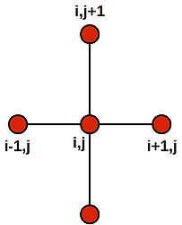
Stencil for a 2D finite difference approximation to the 2nd differential
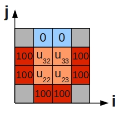
Grid for 2D heat equation


Access patterns with the above 'stencil'--such as that required to solve the 2D heat equation are also prone to thrash the cache, when the size of the arrays are large (800x800 doubles, run on my desktop machine):
performance assessment     LCPI good......okay......fair......poor......bad....
* overall                :  1.3 >>>>>>>>>>>>>>>>>>>>>>>>>>
upper bound estimates
* data accesses          :  6.4 >>>>>>>>>>>>>>>>>>>>>>>>>>>>>>>>>>>>>>>>>>>>>>+
   - L1d hits            :  1.1 >>>>>>>>>>>>>>>>>>>>>>>
   - L2d hits            :  0.5 >>>>>>>>>>>
   - L2d misses          :  4.7 >>>>>>>>>>>>>>>>>>>>>>>>>>>>>>>>>>>>>>>>>>>>>>+
* instruction accesses   :  5.2 >>>>>>>>>>>>>>>>>>>>>>>>>>>>>>>>>>>>>>>>>>>>>>+
   - L1i hits            :  5.2 >>>>>>>>>>>>>>>>>>>>>>>>>>>>>>>>>>>>>>>>>>>>>>+
   - L2i hits            :  0.0 >
   - L2i misses          :  0.0 >
Another good example of thrashing the cache can be seen for a simple looping situation. A loop order which predominately cycles over items already in cache will run much faster than one which demands that cache is constantly refreshed. Another point to note is that cache size is limited, so a loop cannot access many large arrays with impunity. Using too many arrays in a single loop will exhaust cache capacity and force evictions and subsequent re-reads of essential items.
As as example of adhering to the principle of spatial locality, consider two almost identical programs (loopingA.f90 and loopingB.f90). You will see that inside each program a 2-dimensional array is declared and two nested loops are used to visit each of the cells of the array in turn (and an arithmetic value is dropped in). The only way in which the two programs differ is the order in which the cycle through the contents of the arrays. In loopingA.f90, the outer loop is over the rows of the array and the inner loop is over the columns (i.e. for a given value of ii, all values of jj and cycled over):
  do ii=1,nRows
     do jj=1,nCols
        data(ii,jj) = (ii+jj)**2.0
     end do
  end do
The opposite is true for loopingB.f90:
  do jj=1,nCols
     do ii=1,nRows
        data(ii,jj) = (ii+jj)**2.0
     end do
  end do
Let's compare how long it takes these two programs to run:
cd ../example2
make
$ ./loopingA.exe
 elapsed wall-clock time in seconds:   1.2610000
and now,
$ ./loopingB.exe
 elapsed wall-clock time in seconds:  0.41600001
Dude! loopingA.exe takes more than twice the time of loopingB.exe. What's the reason?
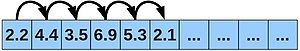
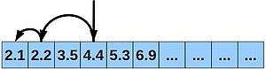
Well, Fortran stores it's 2-dimensional arrays in column-major order. Our 2-dimension array is actually stored in the computer memory as a 1-dimension array, where the cells in a given column are next to each other. For example:

That means is that our outer loop should be over the columns, and our inner loop over the rows. Otherwise we would end up hopping all around the memory, potentially thrashing the cache if the array is large, and using unnecessary time, which explains why loopingA takes longer.
The opposite situation is true for the C programming language, which stores its 2-dimensional arrays in row-major order. You can type:
make testC
To run some equivalent C code examples, where you'll see that an optimising C compiler will spot this mistake and rearrange your loops for you!
Be parsimonious in your data structures
For example:
#define N 1024*1024

struct datum
{
   int a;
   int b;
   int c;  /* Note: unused in loop */
   int d;  /* Note: unused in loop */
};

struct datum mydata[N];

for (i=0;i<N;i++)
{
  mydata[i].a = mydata[i].b;
}
will take longer to run than:
#define N 1024*1024

struct datum
{
   int a;
   int b;
};

struct datum mydata[N];

for (i=0;i<N;i++)
{
  mydata[i].a = mydata[i].b;
}
simply because the second program refreshes cache fewer times.
Avoid Expensive Operations
It's possible that your use of the memory hierarchy is as good as it can be and that your problem is that you are using many expensive operations in your calculations.
- If you are writing code in a language such as Python, R or Matlab, you should be aware that calling functions in those languages will be fast, but writing significant portions of control flow code--loops, if statements and the like--will be slow.
- Beit in a compiled or scripting language, memory operations (such as allocate in Fortran, or malloc in C) are always expensive, so use them sparingly.
- Some mathematical functions are more expensive than others. See if you can re-phrase your maths so that operations such as sqrt, exp and log and raising raising numbers to a power are kept to a minimum.
Make Sure that Your Code 'Vectorises'
Relatively little support if offered to the programmer on this topic. However, since pretty much all modern processors use wide registers, it is a key factor. Furthermore, the trend is toward wider registers (and further chipset extensions) and so the imperative of writing vectorisable code will only increase.
If we consider a loop, wide registers can only be exploited if several of the iterations can be performed at the same time. We must thus ensure that no dependencies exist between loop iterations. For example the value of array index i must not depend upon the value i+1.
Note that the term vectorisation means a slightly different thing when used in the context of scripting languages such as MATLAB, Python or R. In this context, the term refers to the replacement of loops with calls to routines which can take vectors or matrices as arguments. This manoeuvre effectively takes the loop out of the slower interpreted language and executes it in a faster compiled language (since routines in these languages are typically written in C or Fortran).
Scripting Languages
The key steps for optimising programs written in scripting languages, such as MATLAB, Python and R and the same same as for a compiled language: (i) first profile your code; (ii) find the hot spots; (iii) etc. In broad brush terms, the main approach to speeding-up slow portions of code--common to all--is to replace loops with build-in or contributed functions (which essentially outsource the loop to a compiled language, such as C or Fortran).
MATLAB
For and example of using the MATLAB profiler, adding timing code and some hints and tips on writing faster MATLAB code, see the Starting MATLAB course.
See also the Mathworks pages:
- See http://www.mathworks.co.uk/help/matlab/ref/profile.html
- See also tic, toc timing: http://www.mathworks.co.uk/help/matlab/ref/tic.html
R
To see how to use the R profiler and some hints and tips on writing faster R code, see the Starting R course.
Python
In a similar vein, the Starting Python course contains some useful hints, tips and links for profiling and optimising python code.
Scripting Languages vs. Compiled Code
Scripting languages are usually run through an interpreter rather than being compiled into a machine code which is specific to a particular processor, O/S etc. Interpreted instructions often run more slowly than their compiled counterparts. As an example to show how much slower loops are in a scripting language compared to a compiled language consider the following programs, which solve an Ordinary Differential Equation (ODE) initial value problem associated for a damped spring using the (4th order) Runge-Kutta method.
(See, e.g.:
- http://en.wikipedia.org/wiki/Runge%E2%80%93Kutta_methods
- http://mathworld.wolfram.com/Runge-KuttaMethod.html
for more information on the Runge-Kutta method.)
First, rk4.py:
#!/usr/bin/env python

# http://doswa.com/2009/04/21/improved-rk4-implementation.html
# python example.py > output.dat
# gnuplot
# plot 'output.dat' using 1:2 with lines
# should see a nice damped plot

import numpy

def rk4(x, h, y, f):
        k1 = h * f(x, y)
        k2 = h * f(x + 0.5*h, y + 0.5*k1)
        k3 = h * f(x + 0.5*h, y + 0.5*k2)
        k4 = h * f(x + h, y + k3)
        return x + h, y + (k1 + 2*(k2 + k3) + k4)/6.0

def damped_spring(t, state):
        pos, vel = state
        stiffness = 1
        damping = 0.05
        return numpy.array([vel, -stiffness*pos - damping*vel])

if __name__ == "__main__":
	t = 0
	dt = 1.0/100
	state = numpy.array([5, 0])
	print('%10f %10f' % (t, state[0]))

	while t < 100:
		t, state = rk4(t, dt, state, damped_spring)
		print('%10f %10f' % (t, state[0]))
This is a beautifully simple program where the code reads much like the mathematical equations being solved. One of the reasons that the code reads so well is because Python, as a higher-level language, offers features such as a vector, which we can apply the '*' and '/' operators, resulting in element-wise arithmetic. These features are not available in plain C code, and as a consequence the program is a good deal harder to read. rk4.c:
/*
** Example C code to plot 4th order Runge-Kutta solution
** for a damped oscillation.
** Usage:
** $ rk4.exe > out.dat
** $ gnuplot
** > plot 'out.dat' using 1:2 with lines
*/

#include <stdio.h>
#include <stdlib.h>
#include <math.h>

#define N 2 /* number of dependent variables */
#define STIFFNESS 1.0
#define DAMPING 0.05
#define TIMESTEP 1.0/100.0

void rk4(double x, double h, double y[], double(*f)(double, double[], int))
{
  int ii;
  double t1[N], t2[N], t3[N];           /* temporary state vectors */
  double k1[N], k2[N], k3[N], k4[N];

  for(ii=0;ii<N;ii++) t1[ii]=y[ii]+0.5*(k1[ii]=h*f(x,     y,  ii));
  for(ii=0;ii<N;ii++) t2[ii]=y[ii]+0.5*(k2[ii]=h*f(x+h/2, t1, ii));
  for(ii=0;ii<N;ii++) t3[ii]=y[ii]+    (k3[ii]=h*f(x+h/2, t2, ii));
  for(ii=0;ii<N;ii++) k4[ii]=                  h*f(x+h,   t3, ii);

  /* new position and velocity after timestep, h */
  for(ii=0;ii<N;ii++) {
    y[ii] += (k1[ii] + 2*(k2[ii] + k3[ii]) + k4[ii]) / 6.0;
  }
}

double damped_spring(double t, double y[], int ii)
{
  double stiffness = STIFFNESS;
  double damping = DAMPING;
  if (ii==0) return y[1];
  if (ii==1) return -stiffness*y[0] - damping*y[1];
}

int main(void)
{
  double t = 0.0;                   /* initial time */
  double dt = TIMESTEP;             /* timestep */
  double y[N] = { 5.0, 0.0 };       /* initial state [pos,vel] */
  printf("%10f %10f\n", t, y[0]);   /* will plot position over time */

  while (t < 100.0) {
    rk4(t, dt, y, damped_spring);   /* calc new y */
    t += dt;                        /* increment t */
    printf("%10f %10f\n", t, y[0]); /* write out new pos at time t */
  }

  return EXIT_SUCCESS;
}
The C code is clearly a good deal more convoluted than its Python counterpart. However, at runtime:
$ time ./rk4.py > out.dat

real	0m1.386s
user	0m1.108s
sys	0m0.020s
$ gcc -O3 rk4.c -o rk4.exe
$ time ./rk4.exe > out.out

real	0m0.015s
user	0m0.016s
sys	0m0.000s
we see that the C code runs almost 100 times quicker than the Python script!
The readability objection to C can be countered somewhat using C++, rk4.cc:
// Example C++ code for 4th order Runge-Kutta solution for a damped oscillation.
// Usage:
// $ rk4.exe > out.dat
// $ gnuplot
// > plot 'out.dat' using 1:2 with lines

#include <iostream>
#include <valarray>
#include <cstdlib>

#define N 2             // number of dependent variables
#define STIFFNESS 1.0
#define DAMPING 0.05
#define TIMESTEP 1.0/100.0

using namespace std;

valarray<double> rk4(double x, double h, valarray<double> y, valarray<double>(*f)(double, valarray<double>))
{
  valarray<double> k1(N), k2(N), k3(N), k4(N);

  k1 = h * f(x, y);
  k2 = h * f(x + 0.5*h, y + 0.5*k1);
  k3 = h * f(x + 0.5*h, y + 0.5*k2);
  k4 = h * f(x + h, y + k3);

  return y + (k1 + 2*(k2 + k3) + k4) / 6.0;
}

valarray<double> damped_spring(double t, valarray<double> y)
{
  double stiffness = STIFFNESS;
  double damping = DAMPING;
  valarray<double> retval(N);
  retval[0] = y[1];
  retval[1] = -stiffness*y[0] - damping*y[1];

  return retval;
}

int main(void)
{
  double t = 0.0;                     // initial time
  double dt = TIMESTEP;               // timestep
  double state[N] = { 5.0, 0.0 };     // initial state [pos,vel]
  valarray<double> y (state,N);

  cout << t << " " << y[0] << endl;   // write out time and position

  while (t < 100.0) {
    y = rk4(t, dt, y, damped_spring); // calc new y
    t += dt;                          // increment t
    cout << t << " " << y[0] << endl; // write out new pos at time t
  }

  return EXIT_SUCCESS;
}
We do pay a performance price again, however--albeit with much more favourable ratio. The C++ version is ~22 times faster than the Python version (but ~4 times slower than the raw C version.)
$ g++ -O3 rk4.cc -o rk4.exe
$ time ./rk4.exe > out

real	0m0.063s
user	0m0.032s
sys	0m0.032s
Only then Consider Parallel Programming
Writing parallel code is a lot more difficult than writing serial code. Not necessarily because of the new constructs and syntax that you'll need, but because of all the extra pitfalls that exist. There are new bugs to look out for, such as false sharing and deadlock. There is also the potentially performance killing requirements for synchronisation and global operations. If we are to achieve any real benefits from going parallel, we may well need to completely re-design our algorithms so that our programs will scale and not fall foul of Amdahl's Law (http://en.wikipedia.org/wiki/Amdahl's_law).
For an introduction to using OpenMP, see:
For some tips on getting good performance with OpenMP, including how to avoid false sharing, see, e.g.:
Suggested Exercises
See the relevant course material on C, Fortran, MATLAB, Python or R for nuts and bolts advice on getting going in those languages.
- Write a short program (in, e.g. C or Fortran) which highlights the benefits of using compiler flags, such as gcc's -O3, -ffast-math, etc. (Hint a for loop containing some arithmetic will do.)
- Write a short program in the language of your choice which accesses makes a file access during every iteration of a loop. Time it. Now re-write your program to read or write the information from/to memory instead and time it again.
- Write a MATLAB, Python or R script which demonstrates the benefits of vectorisation in one of those languages.
- Write a simple C or Fortran program, using OpenMP, which demonstrates the benefits of work-sharing across a loop.
- Write variations of the above with and without a 'false sharing' bug.