Difference between revisions of "Phase space mode"
| Line 5: | Line 5: | ||
where, C is the cost function value, M is the measured value, m is the model predicted value, n is the normalisation constant, and the suffix i, j, k, refers to the different optimisation datasets. | where, C is the cost function value, M is the measured value, m is the model predicted value, n is the normalisation constant, and the suffix i, j, k, refers to the different optimisation datasets. | ||
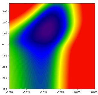
| − | The output from this mode of model run shows the surface of the phase space. In the example below, the response surface for optimising the parameters air temperature lapse rate (<math>\ | + | The output from this mode of model run shows the surface of the phase space. In the example below, the response surface for optimising the parameters air temperature lapse rate (<math>\circ C km^{-1}</math>) [[Image:phasespace_ex.jpg]] |
Revision as of 17:45, 19 November 2007
In this mode the model explores the phase space of the various parameters that are being optimised. The parameter values set in Readoptimfile have boundary values within which parameter values may vary. The subroutine Space_survey runs the model over the range of possible parameter values. For each combination of parameter values a cost function is determined,
[math]\displaystyle{ C = \frac{1}{n_{i}}\sum_{i} \left|{M_{i}-m_{i}}\right|+\frac{1}{n_{j}}\sum_{j} \left|{M_{j}-m_{j}}\right|+\frac{1}{n_{k}}\sum_{k} \left|{M_{k}-m_{k}}\right|+... }[/math]
where, C is the cost function value, M is the measured value, m is the model predicted value, n is the normalisation constant, and the suffix i, j, k, refers to the different optimisation datasets.
The output from this mode of model run shows the surface of the phase space. In the example below, the response surface for optimising the parameters air temperature lapse rate ([math]\displaystyle{ \circ C km^{-1} }[/math]) 